Watch the posterior tighten: a running credible interval with SCAN

Bayes's billiard table ended with a single posterior. Fifty rolls counted, one hump drawn, the hidden ball cornered into a narrow band. That post asked the question fifty times and looked at belief once, at the end. I think the more interesting picture is the one in between, where belief narrows roll by roll, from "anywhere on the table" to "right about here."

Drawing that picture used to be a chore. The cumulative count after look n depends on the count after look n-1, so your options were a column per look, or a chain of cells that each tack on one more term. Both scale badly, and both bury the idea under bookkeeping.

SCAN collapses the whole trajectory into one formula, and MAP turns it into a band. So in this post I rebuild the billiard table as a time series and plot the credible interval shrinking as the evidence comes in.

The cumulative problem

A running total is the simplest case of a pattern spreadsheets handle awkwardly: each output depends on the one before it. That is what SCAN is for. You give it a starting value, an array, and a lambda that folds the next element into the running result. Then it spills every intermediate result, not just the last:

=SCAN(0, A1:A100, LAMBDA(acc, x, acc + x))

That spills the cumulative sum of A1:A100. The first cell is A1, the second is A1+A2, and so on down. acc is the running total, x is the current element, and the lambda body acc + x is the rule. Swap the body for acc * x and you get a cumulative product. Swap it for MAX(acc, x) and you get a running maximum. One formula, one column, the whole trajectory.

If you have run into REDUCE before, SCAN is its sibling. REDUCE keeps only the final fold; SCAN keeps all of them. Both are standard functions, and both survive an .xlsx round trip.

Setting up the rolls

Open a new sheet. As before, hide a ball and roll fifty more. This time, though, pin the randomness with a seed, so the figures in this post are reproducible and the plot stops jittering every time you touch the sheet. (Freeze the dice explains why that matters.)

K1: =SAMPLE.UNIFORM(0, 1, 1, seed=11)        the hidden ball W
A2: =SAMPLE.UNIFORM(0, 1, 50, seed=7)        fifty rolls

K1 is where the first ball comes to rest. We reference it from here on but never read it.

One bit per roll

The billiard post counted all the lefts at once with COUNTIF. To watch belief evolve, we need the per-roll outcome instead: a 1 when a roll lands left of W, a 0 otherwise. MAP applies a lambda to each element of a column and spills the results:

B2: =MAP(A2:A51, LAMBDA(x, IF(x < $K$1, 1, 0)))

Each roll x becomes a single bit. The lambda closes over $K$1, which is to say the hidden position is just a constant the lambda reaches out and reads, the same way any formula reads a cell. No helper column of comparisons, no fill-down.

The cumulative tally

Now SCAN turns the stream of bits into a running count of lefts, and a plain sequence gives the look number:

C2: =SCAN(0, B2:B51, LAMBDA(acc, x, acc + x))     k after each look
D2: =SEQ.LINEAR(1, 50, 50)                          n, the look number

Column C is k, the lefts seen so far. Column D is n, the rolls so far. After roll 1 we have seen one bit. After roll 50 we have the full tally the billiard post computed in a single cell. The difference is that SCAN handed us all fifty intermediate states for the price of one formula.

A band at every step

With a uniform prior, the posterior after k lefts in n rolls is Beta(k+1, n-k+1), and its central 95% runs from the 2.5th to the 97.5th percentile of that Beta. The billiard post evaluated those percentiles once, with scalar arguments. We want them at every look, so we wrap the same scalar BETA.INV in a MAP over the k and n columns:

E2: =MAP(C2:C51, D2:D51, LAMBDA(k, n, BETA.INV(0.025, k + 1, n - k + 1)))   lower
F2: =MAP(C2:C51, D2:D51, LAMBDA(k, n, BETA.INV(0.975, k + 1, n - k + 1)))   upper
G2: =MAP(C2:C51, D2:D51, LAMBDA(k, n, (k + 1) / (n + 2)))                    mean

MAP with two arrays binds one parameter to each and walks them in step, so k and n land on the cumulative count and the look number from the same row. The body is the formula straight out of the billiard post: BETA.INV(0.025, k+1, n-k+1) for the lower bound, Laplace's rule (k+1)/(n+2) for the mean. The only change is that it runs once per look now instead of once at the end. Three MAPs give three columns: lower bound, upper bound, and posterior mean, each a curve over the fifty rolls.

The whole model is six anchors and a hidden ball:

Cell	Formula
K1	=SAMPLE.UNIFORM(0, 1, 1, seed=11)
A2	=SAMPLE.UNIFORM(0, 1, 50, seed=7)
B2	=MAP(A2:A51, LAMBDA(x, IF(x < $K$1, 1, 0)))
C2	=SCAN(0, B2:B51, LAMBDA(acc, x, acc + x))
D2	=SEQ.LINEAR(1, 50, 50)
E2	=MAP(C2:C51, D2:D51, LAMBDA(k, n, BETA.INV(0.025, k + 1, n - k + 1)))

(Columns F and G repeat E with 0.975 and the mean.)

Looking at the result

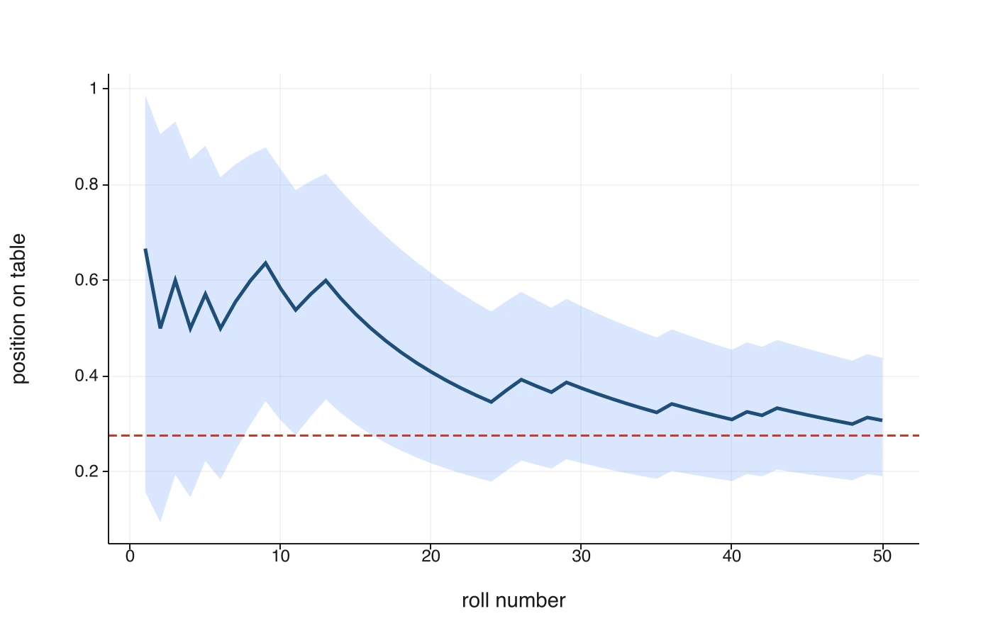
Select the look number (D) as the x-axis and the mean, lower, and upper columns (G, E, F) as three y-series, then draw a line plot. You get the picture you would expect. The mean wanders at first and then settles, wrapped in a band that starts wide enough to cover most of the table and squeezes inward with every roll. Reveal K1 and its value rides inside the band the whole way down, uncertain early and pinned late.

That funnel is Bayesian updating, drawn from the data rather than asserted. Early rolls barely constrain the ball, so the band is loose. Each new bit of evidence tightens it. And the band never collapses to a point, because fifty rolls is only fifty rolls. The width left at the bottom is the uncertainty that honestly remains.

Try it yourself

• More rolls. Change A2 to draw 500 and extend the ranges. The band starts the same and ends far tighter. The funnel just runs longer.
• A different rule. Point the SCAN body at a column of dollar amounts and you have a cumulative cash-flow curve. Point it at returns and you have a running total. The cumulative machinery does not care what it is counting.
• Re-roll reproducibly. Bump the seed on A2 from 7 to 8 for a fresh run you can still reproduce. With the seed in place, the plot you publish is the plot you will see when you reopen the file.

Two new functions did the work here. SCAN carried state down the column so each look could build on the last, and MAP lifted a scalar formula across the whole trajectory. Neither needed a helper column, and both come back intact when you export to .xlsx.