Bayesian updating with grid approximation in TukeySheets

Bayesian inference has a reputation for being intimidating — integrals, conjugate priors, MCMC samplers. But the core idea fits on a napkin, and it fits even better in a spreadsheet. In this post we'll walk through grid approximation, the simplest possible way to do Bayesian updating, using TukeySheets as our scratchpad. The whole model is five anchored spill formulas — no fill-down anywhere, no scratch cells.

The setup

You flip a coin 10 times and get 7 heads. Is the coin fair?

Rather than asking for a single answer, Bayesian inference asks: given what we saw, what's the full distribution of plausible values for the coin's bias p?

Grid approximation answers this in four steps:

Lay out a grid of candidate values for p.
Assign each one a prior probability.
Compute the likelihood of the observed data under each candidate.
Multiply, normalize, done. That's the posterior.

Building it in TukeySheets

Open a new sheet. Put a header in row 1 of each column (p, prior, likelihood, unnorm, posterior) and then drop one spill formula at the top of each data column. TukeySheets's spill engine fans each formula down the column automatically.

Parameter cells — the observed data

Before any formulas, put the observed data in its own labeled cells off to the side so it isn't hard-coded into the likelihood. Pick an unused block:

Cell	Contents
`J1`	`heads` (label)
`K1`	`7`
`J2`	`trials` (label)
`K2`	`10`

Now every formula that needs the data references $K$1 and $K$2. Want to see what 70/100 does to the posterior? Edit one cell, the whole sheet recomputes.

Column A — the grid

In A2, anchor a deterministic sequence spill:

A2: =SEQ.LINEAR(0, 1, 100)

That spills 100 evenly-spaced candidate values for the coin's bias from 0 down through A102. One cell, one formula, no dragging.

Column B — the prior

A flat (uniform) prior says every value of p is equally plausible before we see data. Anchor a spill-vector that broadcasts a constant across the grid:

B2: =A:A * 0 + 1/100

That's the spill-vector grammar from =A:A * 0.5 and friends — A:A auto-sizes to the data rows in column A, so column B always matches column A's length even if you grow the grid.

If you'd rather encode a belief that the coin is probably close to fair, swap in a Beta(2,2) prior in the same anchor:

B2: =BETA.DIST(A:A, 2, 2, FALSE)

We'll keep the flat prior for the walk-through.

Column C — the likelihood

TukeySheets ships the binomial PMF as BINOM.DIST(successes, trials, p, cumulative), and distribution functions vectorize over a range argument — so one anchor covers the whole grid:

C2: =BINOM.DIST($K$1, $K$2, A:A, FALSE)

$K$1 (heads) and $K$2 (trials) point at the parameter cells, and FALSE asks for the PMF rather than the CDF. No hand-rolled p^7 * (1-p)^3, no C(10,7) term to track — the function handles both, and the spill machinery handles the column.

Column D — unnormalized posterior

Prior times likelihood. Pure arithmetic on two ranges, so this is a textbook spill-vector:

D2: =B:B * C:C

Column E — posterior

Divide each unnormalized value by the column sum so the posterior integrates to 1:

E2: =D:D / SUM(D:D)

SUM(D:D) is a scalar reducer; dividing a spill-vector by a scalar broadcasts cleanly. Column E recomputes the moment column D changes.

Aside: SOFTMAX as a shortcut. Normalizing a vector of non-negative numbers to sum to 1 is so common that TukeySheets has it as a single function: =SOFTMAX(D:D) gives the same result as =D:D / SUM(D:D) here.

That's the whole model — five anchors:

Cell	Formula
`A2`	`=SEQ.LINEAR(0, 1, 10n)`
`B2`	`=A:A * 0 + 1/100`
`C2`	`=BINOM.DIST($K$1, $K$2, A:A, FALSE)`
`D2`	`=B:B * C:C`
`E2`	`=D:D / SUM(D:D)`

Looking at the result

Select columns A and E, open the plot editor, and draw a line plot with p on the x-axis and posterior on the y-axis. You'll see a smooth bump peaking near p = 0.7 — exactly the maximum-likelihood estimate — but with real uncertainty spread out roughly between 0.4 and 0.9.

That spread is the whole point. A frequentist would report p̂ = 0.7. The Bayesian posterior tells you there's still meaningful probability that the true bias is 0.5 (a fair coin), and the data alone isn't enough to rule that out.

Updating sequentially

The real magic of Bayesian thinking: yesterday's posterior is today's prior. Flip 10 more coins, get 6 heads. Park the new batch in its own parameter cells (K3 = 6, K4 = 10, with labels in J3/J4) and add three more anchored spills in columns F, G, H:

F2: =BINOM.DIST($K$3, $K$4, A:A, FALSE)    new likelihood
G2: =E:E * F:F                              posterior-as-prior × new likelihood
H2: =G:G / SUM(G:G)                         renormalize

Plot column H next to column E and you can see the update unfold panel-by-panel:

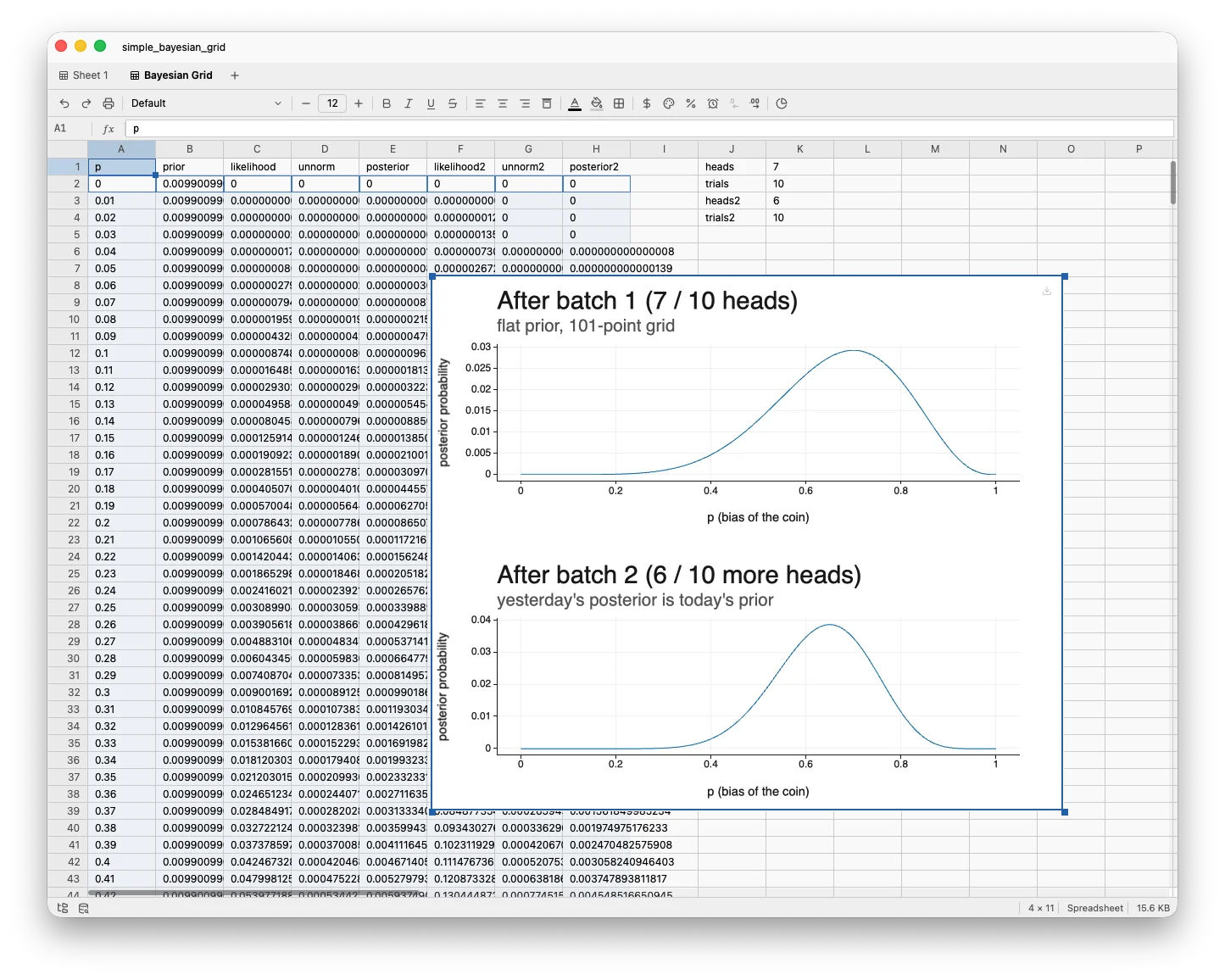
The bump tightens and shifts slightly. Each batch of data narrows your beliefs, and each update is one more block of three spills.

Why this matters

Grid approximation doesn't scale — with two unknown parameters you'd need a 2D grid, with five unknowns the grid explodes. That's why MCMC exists.

But for understanding what Bayesian updating actually does, nothing beats watching numbers multiply, sum, and renormalize in front of you. The whole pipeline — prior, likelihood, posterior — sits on one screen as five formulas. No black boxes, no samplers, no diagnostics. Just arithmetic over columns.

And when you're sanity-checking a fancier model later, the grid version in a TukeySheets tab is the friend who'll tell you when you've made a sign error.

Try it yourself

Change the prior anchor in B2 to a Beta(2,2): =BETA.DIST(A:A, 2, 2, FALSE). The rest of the sheet recomputes automatically.
Change the data by editing K1 and K2. What if you saw 70 heads in 100 flips? The likelihood, posterior, and plot recompute the instant you press enter.
Tighten the grid: bump SEQ.LINEAR(0, 1, 100) to SEQ.LINEAR(0, 1, 1001). Every downstream spill auto-resizes — A:A references take care of it.

That's Bayesian updating. One column at a time, one anchor per column.